
This blog post is part of a “Statistical Hypothesis Essentials”series of stories about the basics of hypothesis testing, and its vocabulary. To immediately receive a post when it’s out, subscribe to my Substack.
📮 Make sure you don’t miss out! Follow this blog and subscribe to an e-mail list to ensure you are among the first to get the article! Please check the rest of the website for detailed articles, cheat sheets, glossaries, and case studies.
Make sure to also download the cheat sheet based on this – click here.
In this series, I’m covering the topic of hypothesis testing, and how to proceed with it in an R environment. Last time I talked about what hypothesis testing is, and what are the crucial parts of it. In this article, I will discuss more appropriate tests you can select, their assumptions, and what to do when those assumptions are unmet.
HYPOTHESIS TESTING — WHAT IS IT?
As I said in the earlier article, hypothesis testing is one of the most used statistical methods, being a part of inferential statistics. It comprises null and alternative hypotheses, alpha level, and test statistics. The testing itself has its assumptions like normality and independence of observations, but it is important to clarify the assumptions of test statistics as well.
IMPORTANCE OF TEST STATISTICS IN HYPOTHESIS TESTING
Test statistics is used to measure how far away the sample data deviates from the null hypothesis. The choice of which test statistics you will choose depends on multiple things, such as:
- type of data
- sample size
- assumptions are met — normality, equal variances…
To calculate a test statistic, follow this procedure:
- formulate both hypotheses
- and collect the sample data — that will allow you to do hypothesis testing. Make clear goals for the sample collection.
- choose the appropriate test — perform EDA and evaluate your data. Your data should be at least checking the normality prerequisite, as that is a prerequisite for almost all tests. If your EDA shows outliers, you should see why they happen, evaluate them, and decide on what to do with them (to standardize data, log the data, delete the outliers…). Check this article to see all the options and how to identify outliers.
- calculate the test statistic — use the formula that is specific to the chosen test and calculate it based on sample data and the variables.
TESTS IN HYPOTHESIS TESTING PROCESS
There are a few tests that you can use in hypothesis testing, but the most used ones are:
1. z-test
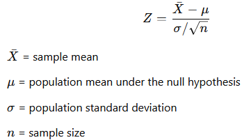
You might hear about standardization and z-scores, and this test makes you believe it might be on the same lane. It is used when the sample size is large (n>30) and the population standard deviation is known. When you are performing your research, you might use this test as you know out of which population you took the sample, or the population is quite small (i.e. all students at college XY).
This test is used to determine if there is a difference between the sample’s and the population’s mean, or between the means of two samples. It is based on z-distribution which is another name for a standard normal distribution (hence the name z-test).
It can be one-sample, two-sample, or z-test for proportions.
Assumptions to use this test are the following:
- sample size has to be greater than 30
- the population’s standard deviation is known
- the data has to be approximately normally distributed
Most of the time, the population’s standard deviation is not known and it is not smart to just presume it, or fake that you know it, as it can distort the whole testing process. If you would like to calculate it manually, then this is the formula for it:
In R environment, there are two ways to calculate it:
a. putting this manual formula in R:
z_test=(sample_mean - population_mean) / (population_sd / sqrt(sample_size))
print(z_test)
b. download an appropriate package and perform a z test:
library(BSDA)
#prepare the sample data and attach it
ztest=z.test(sample,mu=XY,sigma.x=YX)
print(ztest)

#mu is the population mean
#sigma.x is the known population standard deviation
2. t-test
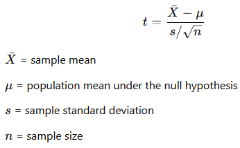
The most used test statistic is the t-test, as most of the datasets we find only are not quite clear about their population, or the parameters of the population are not that easy to find. Other than that, it is also used when our sample size is very small (n<30). If you would like to calculate it manually, then this is the formula for it:
In the R environment, you can calculate it in the following way:
#prepare the sample data and attach it
ttest=t.test(sample,mu=XY)
print(ttest$statistic)

#mu is the population's mean.
A T-test is a test that we use to determine if a difference between two averages is real or just a coincidence. It takes samples from both groups to determine if there is a difference between the means of the two groups, all while considering the sample size and variability (as you can see in the formula itself). It can be a one-sample, two-sample, and paired-sample t-test.
The test is used when:
- data is on an interval or ratio scale
- data is approximately normally distributed
- the samples are independent or paired (depending on which test you perform)
- the variances of the populations are equal
- the sample size is not too small, aka it has to be larger than 30
In one of the following articles in this series, I will write a detailed article about t-testing, with examples in R.
3. ANOVA
ANOVA test is used to compare means among three or more groups to see if at least one group’s mean is different from the others. It can be one-way or two-way, depending on how many independent variables you use (those independent variables are categorical). It involves calculating the F-statistic, which is the ratio of the variance between the groups to the variance within the groups.
Assumptions of ANOVA are the following:
- the samples are independent of each other
- the data in each group should be approximately normally distributed
- the variances in different groups should be approximately equal
In the R environment, you can calculate it in the following way:
anova=aov(y~x,data=name_of_your_dataset) #for one-way anova
summary(anova)

OR

anova=aov(y~x + z,data=name_of_your_dataset) #for two-way anova
summary(anova)
4. Chi-square test
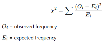
A chi-square test is used for categorical data to assess how likely it is that an observed distribution is due to chance/luck. It evaluates if there is a relationship/correlation/dependence between the categories of the two variables, so we need numerical and categorical variables. Most of the time, those two types of variables create a contingency table.
The test is used when:
- the data is in the form of counts/frequencies for categories
- each frequency should not be less than 5
- the observations should be independent of each other
Manually, you can calculate it in the following way:
Most of the time, you will deal with a greater dataset that will have more numerical and more categorical variables, and you only need a few of them for this test. In that case, you can create a contingency table of your own, like this:
condata=data.frame(dataset_name$x, dataset_name$y)
condata=table(dataset_name$x, dataset_name$y)
Only then you can apply a chi-square test in R, by writing this code:
print(chisq.test(condata))
#this code both calculates the test and prints out the output.
CONCLUSION
Understanding the appropriate hypothesis test and its assumptions is critical for accurate statistical analysis. When assumptions are not met, it is essential to use alternative methods to ensure the validity of your results, such as non-parametric tests which are used when the data is not normally distributed, or there is a small sample size. By carefully considering these factors, you can make more informed decisions and draw more reliable conclusions from your data.
Make sure to follow my website, as I will publish detailed articles about each of these tests. Once they are written, I’ll make sure to update this article with the links.
Follow this blog and subscribe to an e-mail list to ensure you are among the first to get the article!
